5th Week, 3D scanning and printing
This week we focused on 3d printing and scanning. Both subjects are so broad I could spend more than a week on each one, but I tried to do as much as possible in the time I had.
3d Printing
3D printing, also known as additive manufacturing (AM), refers to the process of manufacturing a three-dimensional object by laying successive layers of material that are solidified to create the object. Objects can be of almost any shape or geometry and are produced using digital model data from a 3D model.
In reality however 3d printing has many constraints in the geometries that can be produced, it has a low structural properties (i.e. it breaks very easily), the finishing in most 3d printers is not very good, it is very slow, and it requires a lot of post processing. What is more, the overhangs of the geometry can not be more than 45 degrees , and sometimes even less depending on the printer and the material, otherwise the print will fail. I must admit I was not a great fan of 3d printing before this week, and I am still not a great fan after this week.
The week started with tests on the tolerances in groups. Here's the group project page where you can find more details about that. The test files we used were downloaded from these sites: 3D Printer Tolerance Test, and Test your 3D printer! v3.
For the group assignment we chose a test model from those websited, in order to try out our printers and evaluate their performance and quality of the prints. The software we used is Cura, a free software that can 3D slice models to be 3d printed for almost every 3d printer. There are many parameters that need to be adjusted for the print to come out well, and we experimented with them in the group assignment. The most important of those are: Layer height , this determines the resolution of the print. Line width, this determines the thickness of the line in width, and its value should be close to the noozle diameter of the printer. Percentatge of infill, this sets up an internal mesh in the object, the more dense it is the object becomes more resistant, but also heavier, longer to print and more expensive to print. Wall thickness, this determines the thickness of the wall, usually it is around 1-2mm and it affects the final strength of the object. Supports, these create some external supports in case there are overlaps with an angle greater than 45 degrees, which would collapse without extra supports. Supports should be avoided if they are not necessary because they increase the time and the material necessary for the print, they are sometimes hard to remove, and they can leave extra marks on the surface of the object after their removal.
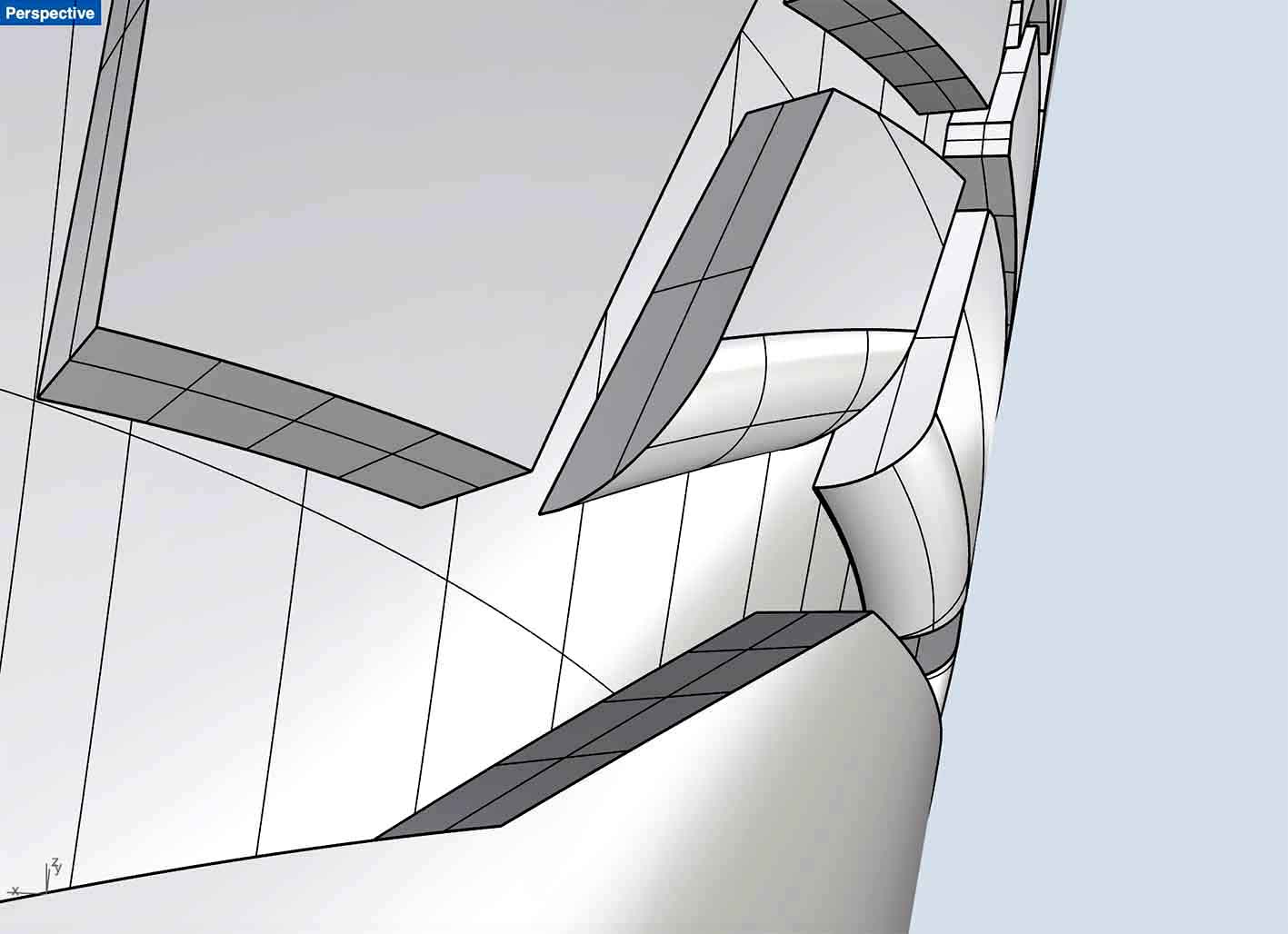
I wanted to produce a complex geometry that could not be manufactured in any other way. I went back to a grasshopper algorithm I was working on a few weeks ago on generating trees (almost) recursively, and I decided to use this design as a pattern to make a 3d printed lamp.
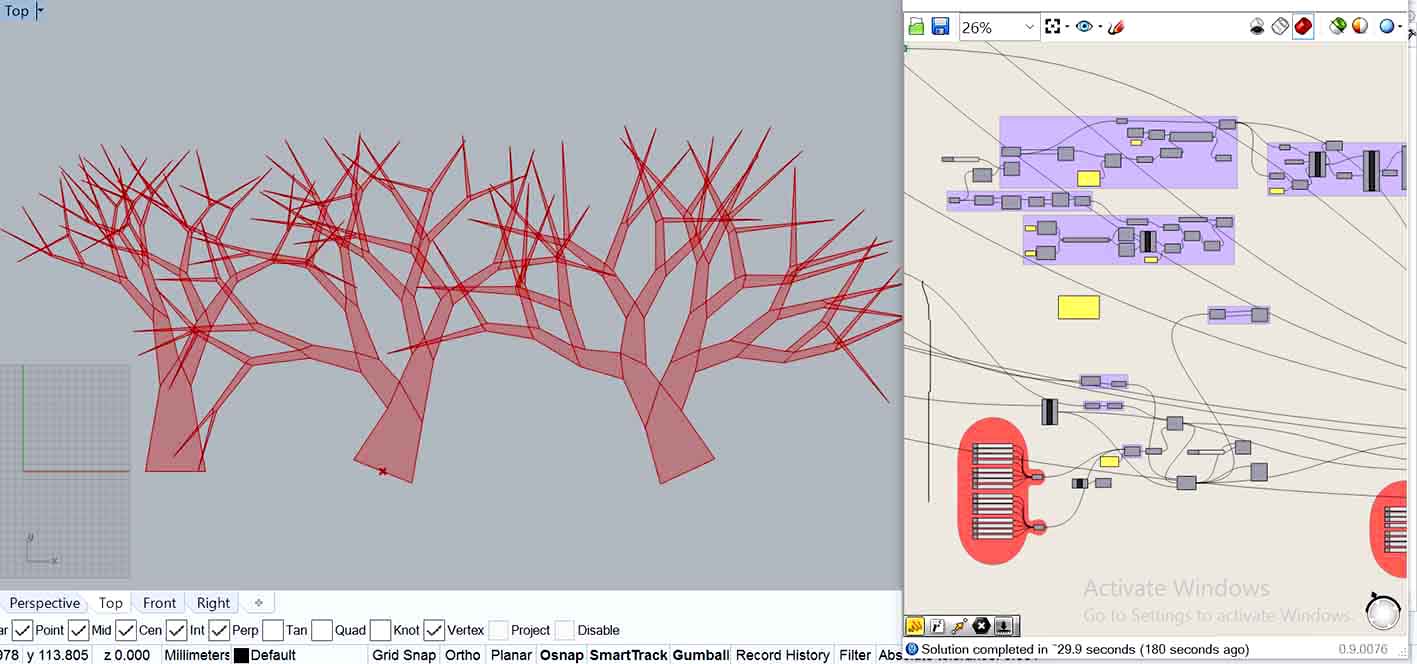
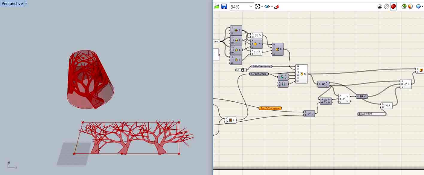
I created a cylindrical surface and wrapped the pattern around it. I then extruded the surfaces in a non-uniform way so that while the z increases, the depth of the extrusion decreases. As a result I had the thicker branches deeper and the thinner branches shallower. After that, a boolean was NOT all it took to subtract the “trees” from the cylindrical surface, but I will not bother you with details here, for more information download the grasshopper file here. Eventually it did work, and here’s the result.
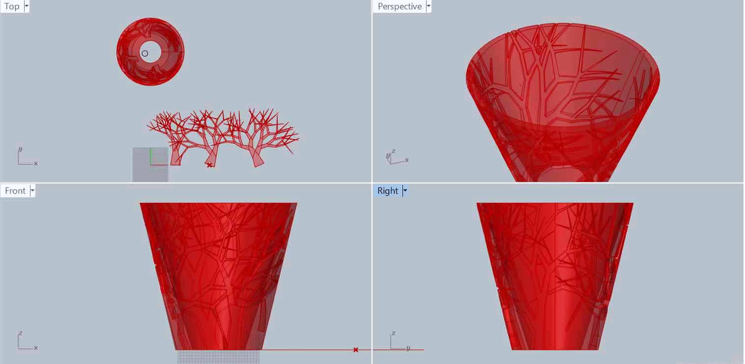
I then baked the geometry in Rhino, but soon I realised, with our wise technician’s advice, that it would probably never print well. So I started deleting the parts that looked to be the most dangerous ones, and filleting wherever I could the horizontal overhangs. It was a long but necessary process, which should optimally have been done in Grasshopper.
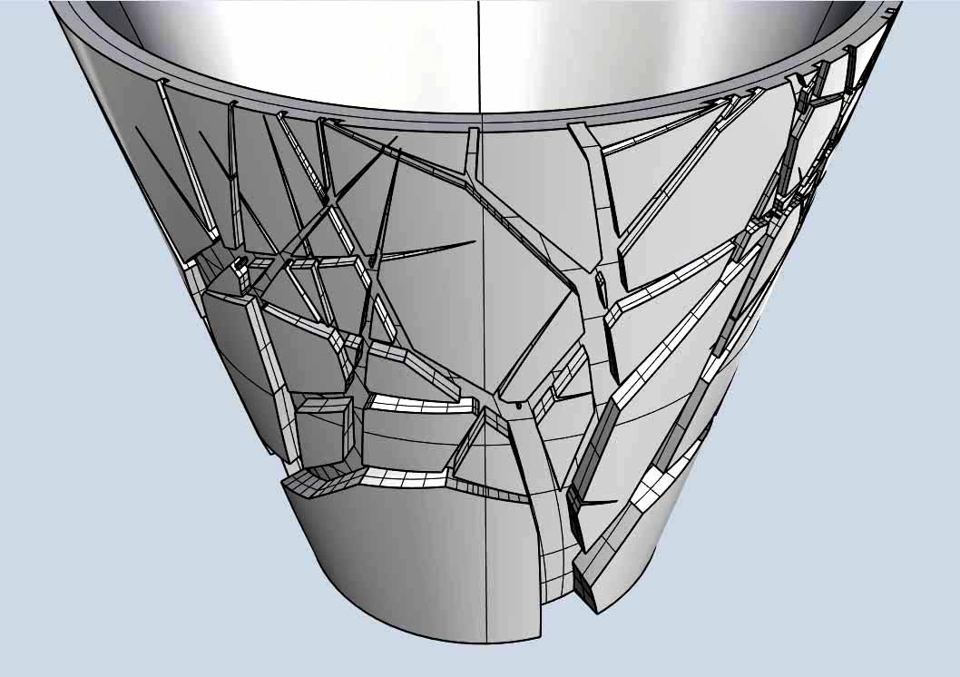
This geometry can not be fabricated subtractively using a 3 axis machine, because it has overhangs. So it must be done on the 3d printer.
The print took more than 10 hours, which was a big disadvantage of this project. It was done in a Rep Rap machine, with a 0,6 nozzle, without supports, with 80% infill (which was a HUGE mistake, it should not have been more than 20%) and on 150% speed.
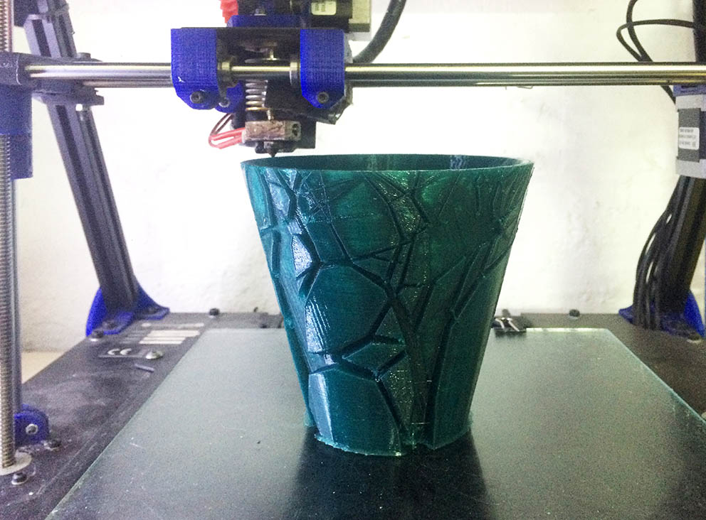
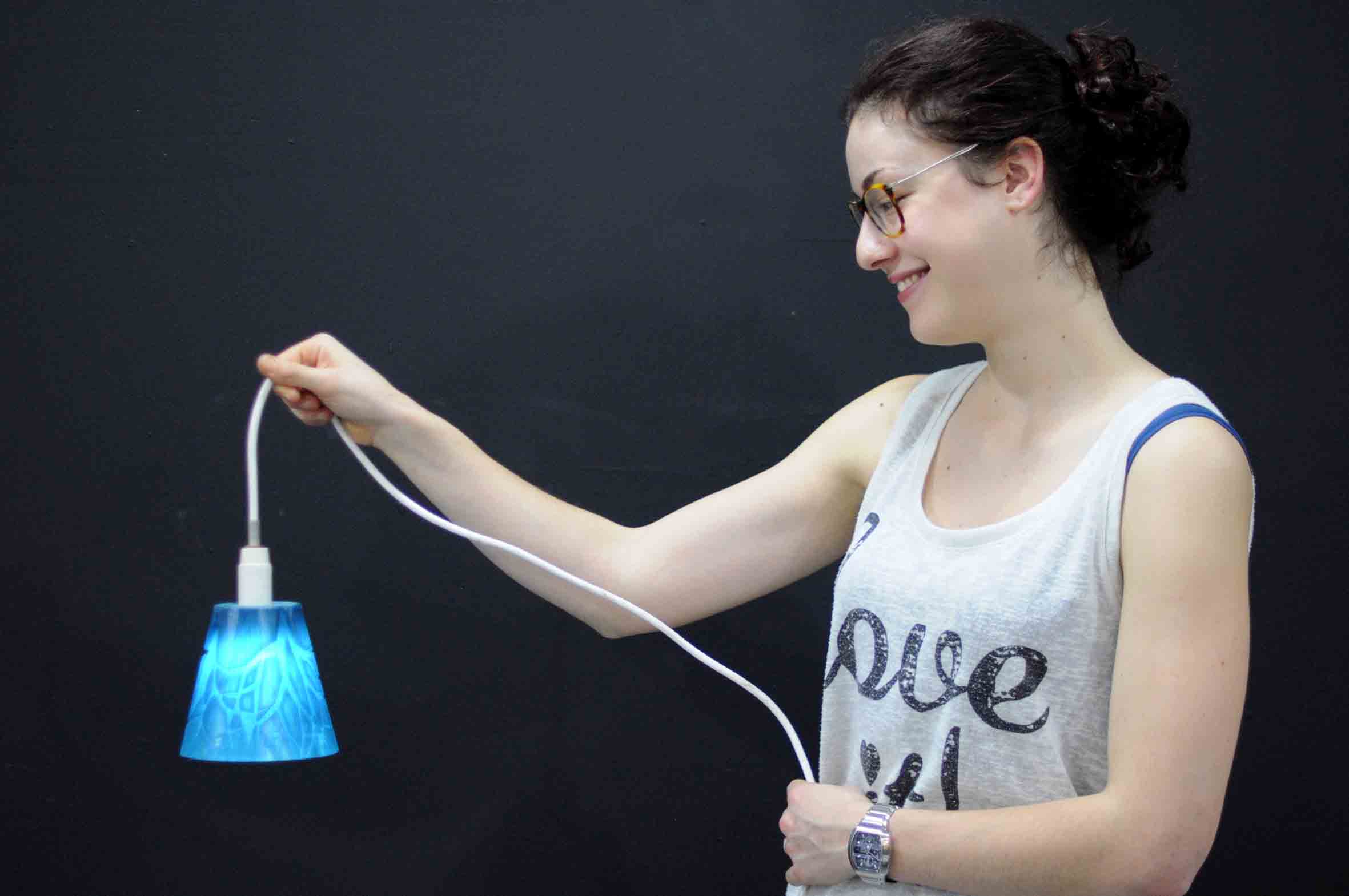
Here’s the final result.
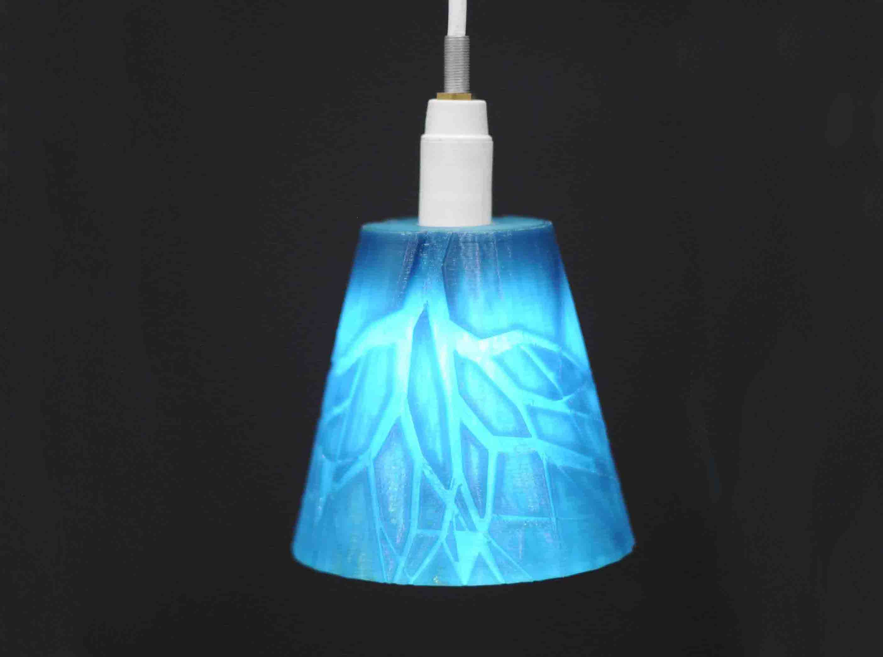
And here you can download the Rhino file.
for this lamp.
And me full of pride
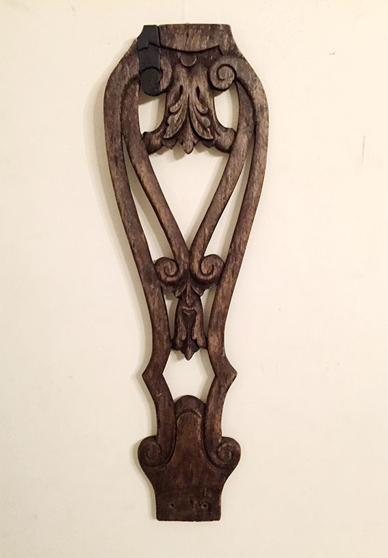
Another small project I undertook was inspired during a walk in the forest around the Green Fab Lab in Valldaura, where I found an old broken piece of wood very elaborately carved which ws missing a little piece. I carefully measured the wood using scanning and orthophotography and I designed and printed the missing piece. This was print on the Ultimaker 2, with 25% infill, 0.4 nozzle, and it took less than 2 hours.
3d Scanning
3D scanning is the process of capturing digital information about the shape of an object with equipment that uses a laser or light to measure the distance between the scanner and the object. The "digital information" that is captured by a 3D scanner is called a point cloud. Each point represents one measurement in space, and they are then connected to form continuous geometry.
The equipment provided for 3d scanning in the lab is a Kinect v1. This was not the first time I use a kinect, but I am not an experienced user either.
I begun by 3d scanning myself on skanect with the help of a friend, and then I 3d printed printed me. For this scanning we used Kinect. I was sitting on a chair that could rotate, and I was rotating slowly trying not to change my position. My friend was standing at the same position, holding the Kinect steadily and moving it slowly up and down as I was rotating.
All it took was a smiley face and two hours of 3d printing.
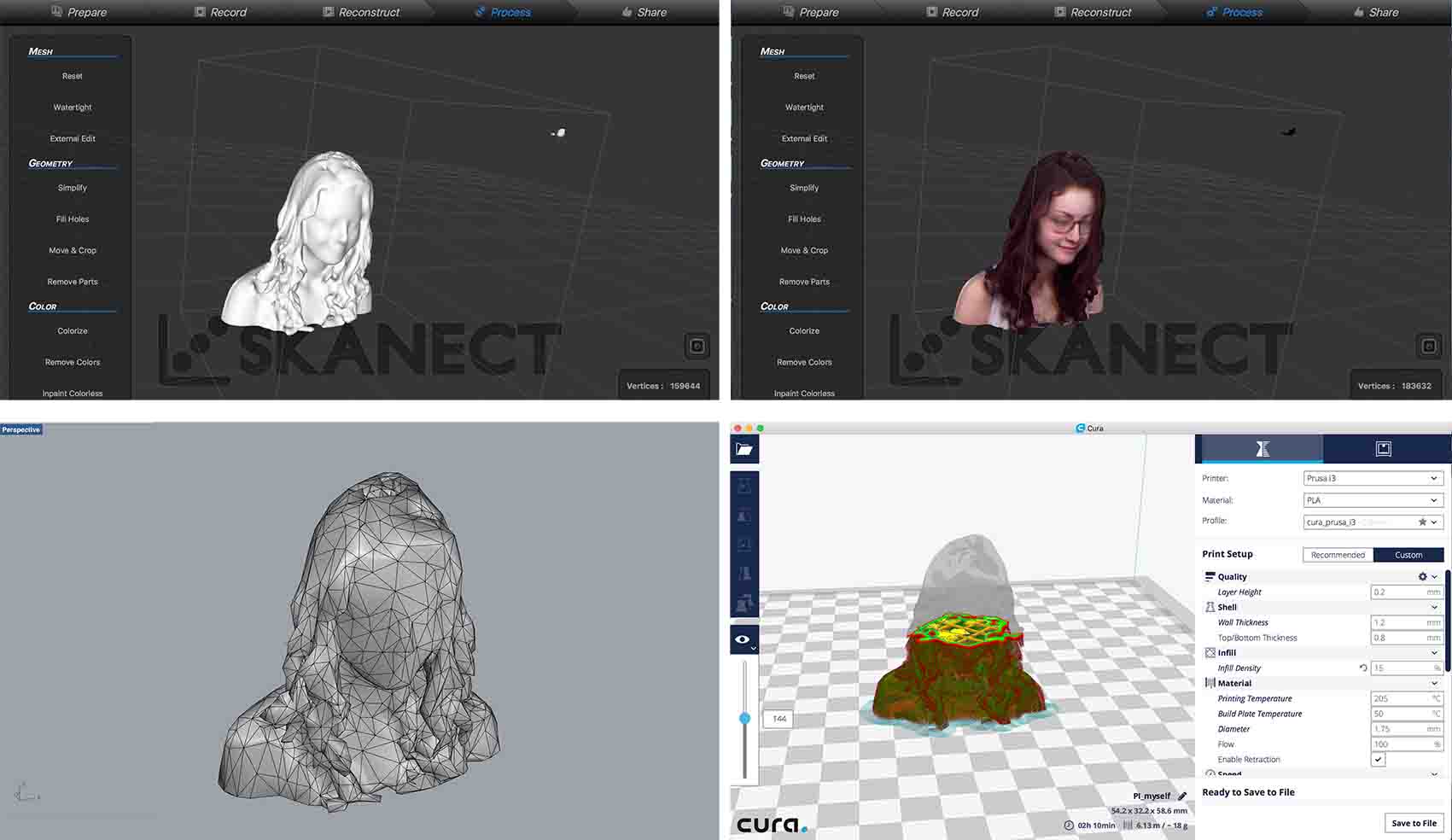
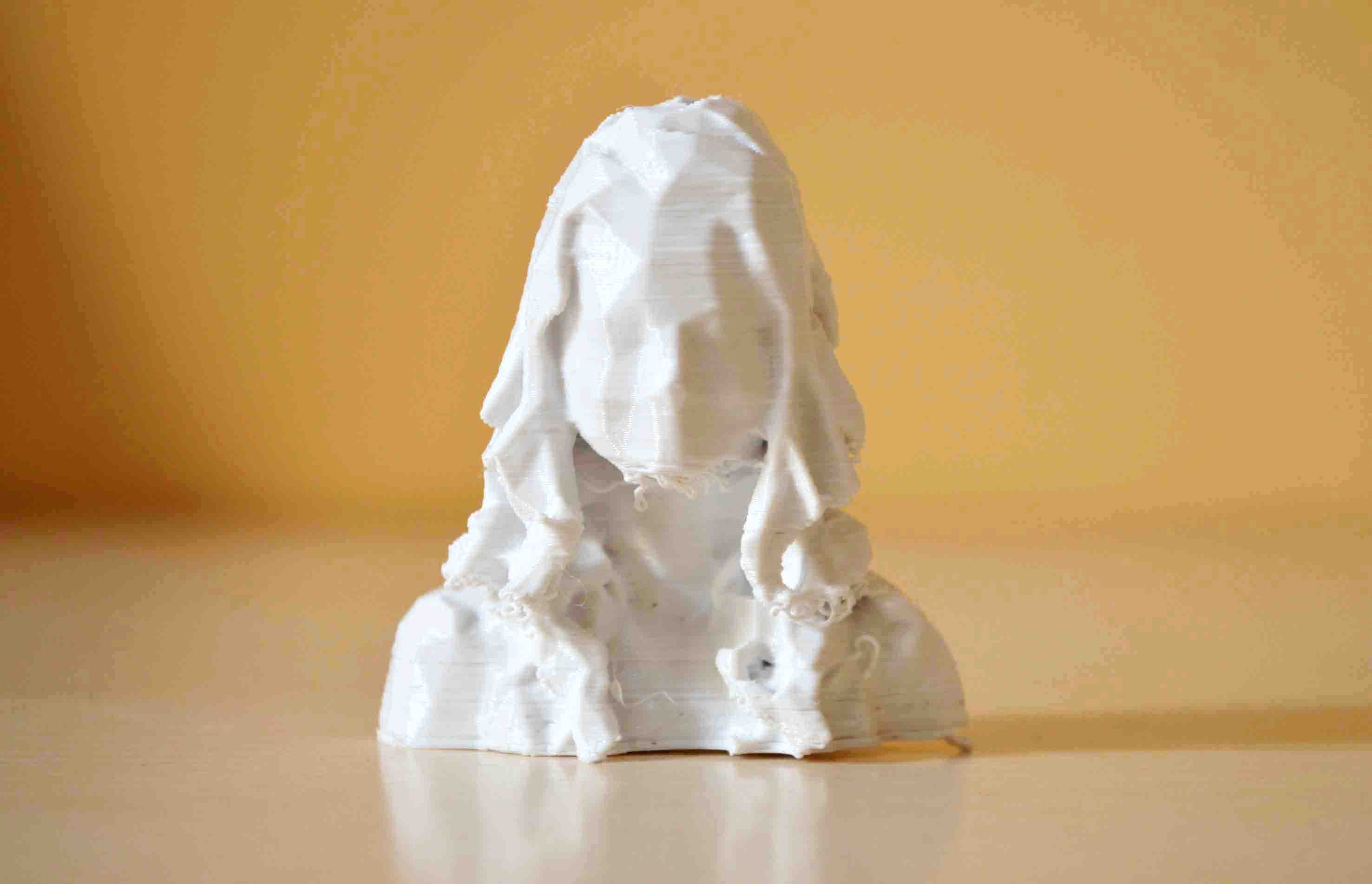
You can download here the result of this 3d scanning as it was when I imported it on Cura for 3d printing: myself.stl. I did not need to fix the model before 3d printing it, I just used the skanect command "Cap holes", and then it became a closed mesh and thus was ready for printing.
Soon I moved on to Processing. I wanted to combine computer’s vision tracking with the kinect’s depth sensor.
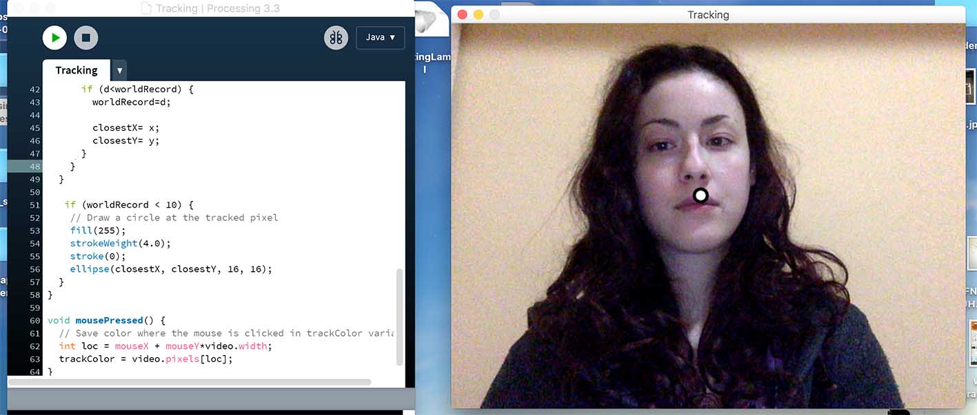
I started working on vision tracking alone. My basic reference for that was Daniel Shiffman’s tutorials to which I link below, and my only equipment the web camera of my laptop.
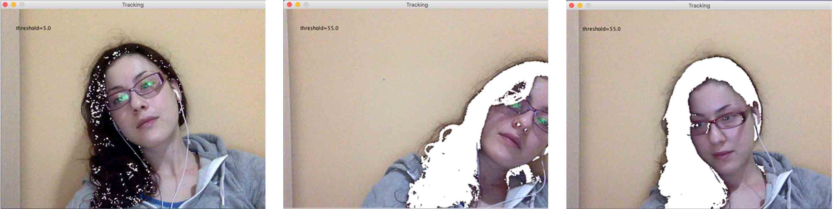
When I felt comfortable with that, I started working with the OpenKinect Library for Processing. I experimented with different settings for tracking and visualisation using the raw depth data and the depth image.
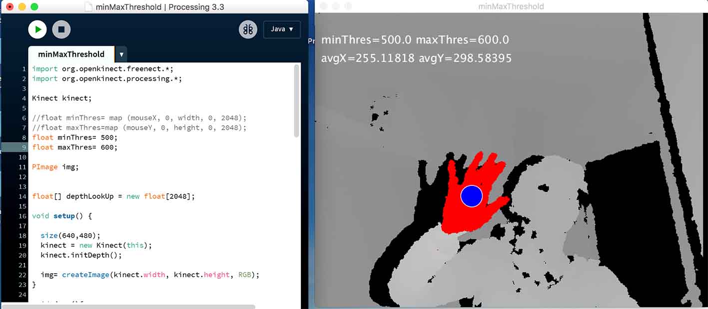
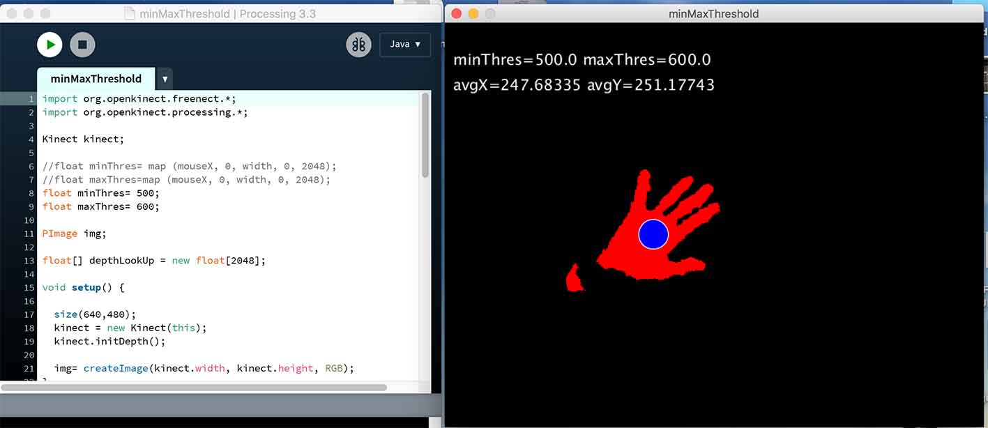
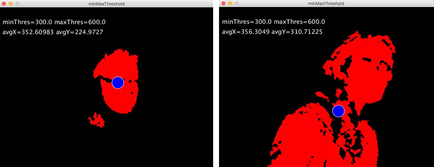
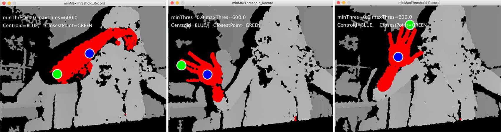
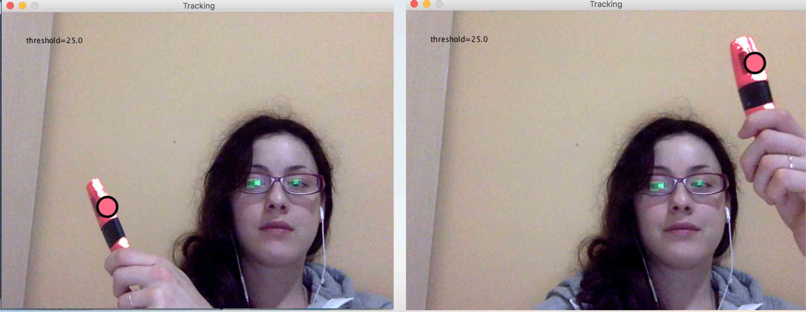
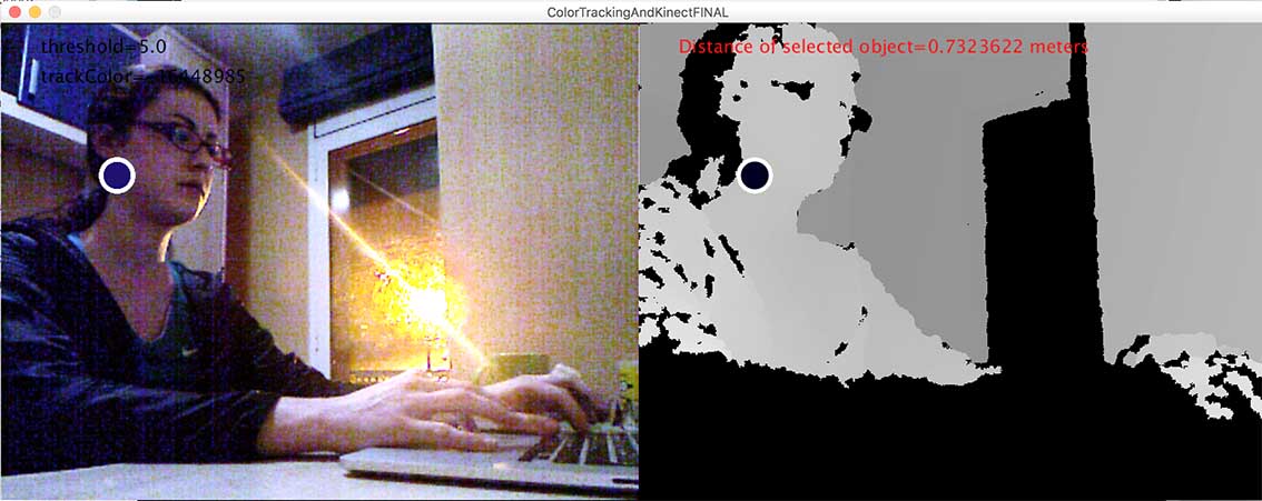
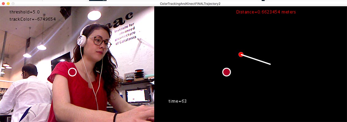
Finally I put together computer vision tracking and openKinect, and wrote a sketch hoping to do the following: the users clicks on an object on the videocamera image, and then the computer tracks this object from its colour and finds its distance from the Kinect. By storing all the distance and position measurements in arrayLists, the trajectory of that moving object can be calculated, using 3d polar (spherical) coordinate system. In summary, the tracking of the object is done by Kinect’s videocamera alone , and the distance is found by the depth sensor. Then the x,y,z coordinates of the object are calculated and drawn on the screen.
At the moment I have the tracking (sort of) working, which gives me the x,y coordinates on the video image, and I find the distance of the tracked object from the raw depth data. Those 3 values are stored in three ArrayLists in order to be converted into x,y,z of the object. The problem is the translation of this aX, aY and distance data to x,y,z coordinates on the screen. They must first be translated to polar coordinates, and then to cartesian. But for this, different units must be combined: pixels and meters. I am still working on that and it proves to be harder than I expected.
Future Improvements
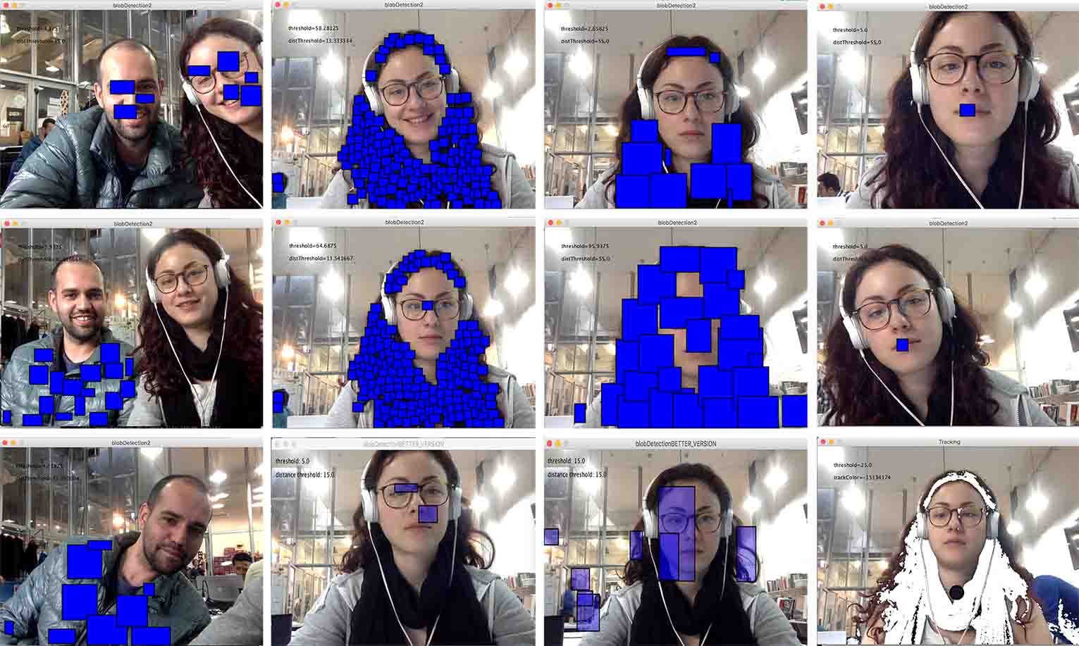
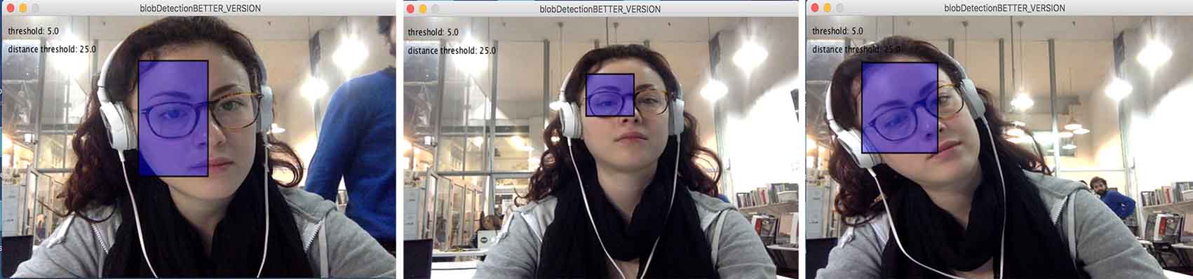
I already mentioned the problem in the conversion of the measurements to x,y,z position of the object which requires further work. Apart from that, the tracking system is also far from perfect, because it only relies of the colour of a few pixels, and so it jumps around introducing a lot of noise. The next step is to implement blob tracking, which is proposed in Shiffman’s tutorials, so that instead of a pixel, a whole area of neighbouring pixels is being tracked. In the future I will use blob tracking and a noise-reduction mechanism with linear interpolation, and of course the possibility to export the geometry in a 3d file.
If you want to download my processing sketch:
Version that is working with 1) tracking and 2) distance but without drawing trajectory, click here.
Version that is with 1) tracking, 2) distance and 3) trajectory, but not working very well, click here.
References
Library for Kinect+Processing: openKinect.orgTutorials on Kinect+Processing by Daniel Shiffman.
Examples of Kinect+Processing by Daniel Shiffman on Github.
Great (!!) tutorials on Computer Vision and Processing, by Daniel Shiffman:
Functions for mapping from the depth camera's (i, j, v) into the world’s coordinates: webpage, by Matthew Fisher